Minimap2 genome alignment tutorial
To quickly run the entire code and have all the input files, clone this repository.
git clone https://github.com/StevenVB12/Tutorial_pan_genomics
To make sure you have everything installed and setup, check here.
1. Introduction
In this tutorial we will align a piece of chromosome of two Heliconius butterfly species that includes the optix gene.
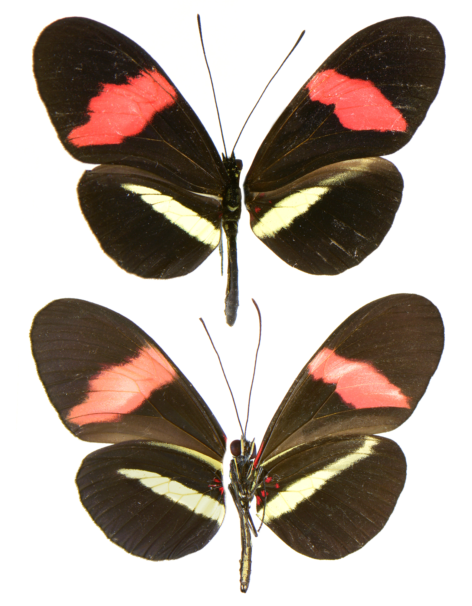
Dorsal (top) and ventral (bottom) sides of Heliconius melpomene rosina (left) and Heliconius erato demophoon (right). The optix gene codes for a transcription factor that plays a key role in the development of red color pattern elements.
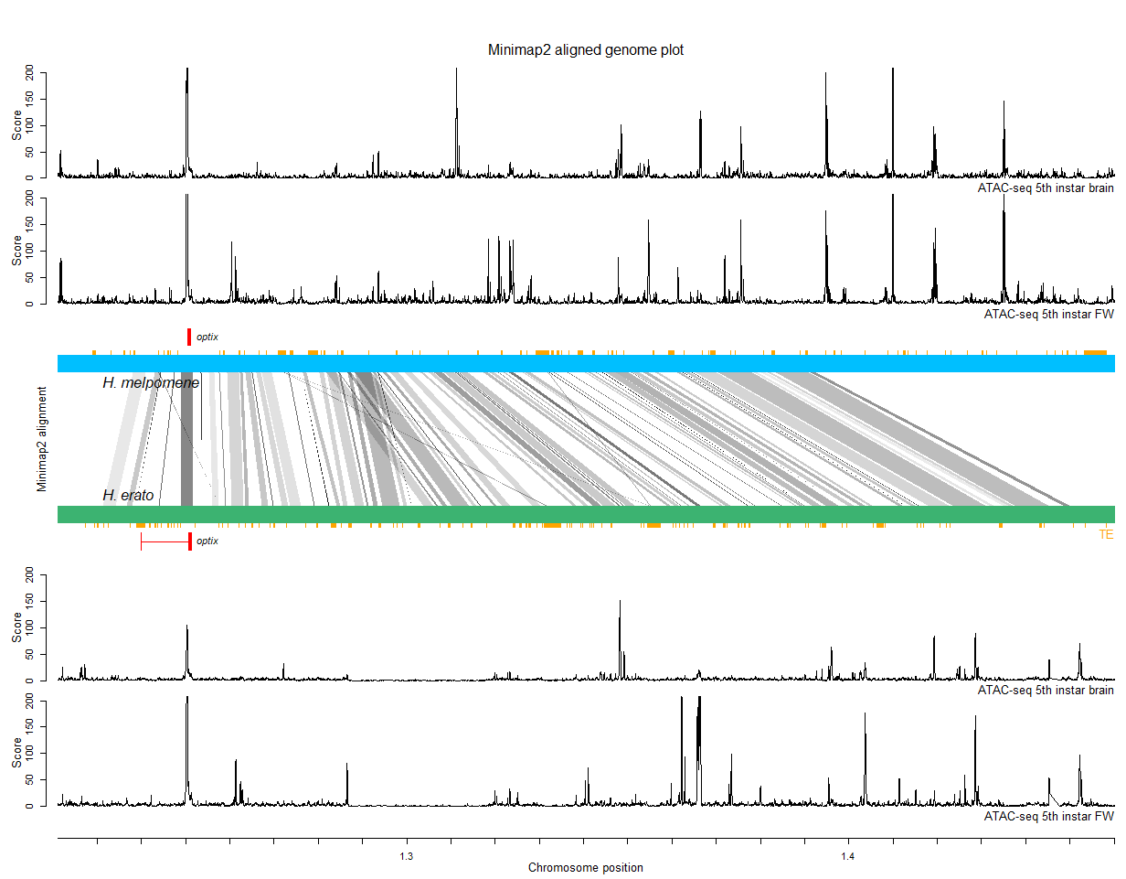
We will use Minimap2 to identify genomic intervals with significant resemblance between the two species and use R to visualize this alignment. Additionally, we will add Transposable Element (TE) annotations and chromatin accessibility profiles (ATAC-seq) of developing head and wing tissues to this plot.
The final result should look like this:
Note: I will sometimes switch between code used in the Linux terminal or Rstudio. I've put these in black and blue boxes, respectively.
2. Input data
For this exercise, you can navigate to http://ensembl.lepbase.org/ and click on the links to the Heliconius erato demophoon (v1) and Heliconius melpomene melpomene (Hmel2) genome assemblies. At the right top, you can search for "optix". The search result will return you the gene model name (e.g. evm.TU.Herato1801.64) and its location (e.g. scaffold 'Herato1801' at position '1239943' to '1251211').
# optix H. erato
Herato1801:1239943-1251211

# optix H. melpomene
Hmel218003:705604-706407
When you click on the gene model, you can see what genes surround the optix gene. You can also see a botton on the left "Export data". This allows you to export the sequence as a .fasta file. Using this, you can try exporting not just the optix gene but a 2,000,000 bp region surrounding it.
You can also find these .fasta files here.
# scaffold Herato1801 start 1 end 2000000
sequences/Herato1801_1_2000000.fasta

# scaffold Hmel213003 start 1 end 2000000
sequences/Hmel213003_1_2000000.fasta
3. Minimap2 aligner
We can use Minimap2 to align the sequences in the fasta files. Minimap2 is intended to efficiently map error prone long-read sequences to a reference (e.g. from nanopore or Pacbio sequencing) but it also works well for pairwise alignment of whole chromosomes and genomes.
For our sequences, we will use Minimap2 as follows:
minimap2 -x asm20 sequences/Hmel213003_1_2000000.fasta sequences/Herato1801_1_2000000.fasta --no-long-join -r 200 | cut -f 1-12 > Minimap2_out/Minimap_melp_erato.sam
Note that we have set here Hmel213003_1_2000000.fasta as the target and Herato1801_1_2000000.fasta as the query sequence.
The -x asm20 option is a preset to optimize alignment of sequences divergent up to 20%. The --no-long-join -r 200 option assures that alignments include no gaps longer than 200 bp (otherwise the result may be one long contiguous alignment). See here for more detailed information on the Minimap2 command.
The | cut -f 1-12 will only take the first twelve columns of the Minimap2 output. This is sent to the file Minimap_erato_melp.sam.
The output should look like this (without the column titles as shown here. See here for more info):
| queryName | queryLength | queryStart | queryEnd | char | targetName | targetLength | targetStart | targetEnd | matchingBases | matchLength | matchQuality |
|---|---|---|---|---|---|---|---|---|---|---|---|
| Herato1801 | 2000000 | 700514 | 710441 | + | Hmel218003 | 1895173 | 228710 | 238849 | 3366 | 10410 | 60 |
| ... | ... | ... | ... | ... | ... | ... | ... | ... | ... | ... | ... |
Note here that the target length isn't actually 2000000 bp but 1895173 bp. That's because the H. melpomene scaffold Hmel218003 with the optix gene has a length of 1895173 bp only.
That's it. For me the alignment step took less than a second. Thanks Heng Li!
4. Visualizations in R
Now we can switch to Rstudio.
4.1. Set you working directory
setwd("G:/My Drive/Workshop_pan_genomics_12042023")
(You can also use the '...' under the 'File' tab on the right of Rstudio to navigate to your folder then click 'More' > 'Set as working directory'.
4.2. Load the Minimap2 output
miniMap_out <- read.table('Minimap2_out/Minimap_melp_erato.sam', header = FALSE, sep = '\t')

# set the column names
colnames(miniMap_out) <- c('queryName', 'queryLength', 'queryStart', 'queryEnd', 'char', 'targetName', 'targetLength', 'targetStart', 'targetEnd', 'matchingBases', 'matchLength', 'matchQuality')

# check the table
head(miniMap_out)
4.3. Plot the first minimap2 match
First, with the rect() function we can define the genomic intervals/sequences of H. melpomene (deepskyblue), the other H. erato (mediumseagreen).
# First define x-axis coordinates. This will help us later define the genomic window (xlim) we want to zoom in on.
start = 0
end = 3000000

# Plot an empty plot (so we can fill it with rectangles (~genome) and polygons (~alignments)).
# For the y-axis (ylim) coordinates I arbitrarily use c(0,10).
plot(NULL, xlim = c(start, end), ylim = c(0,10), axes=F, ylab = '', xlab = '')

# Now we can draw two simple rectangles, one will define the genomic interval/sequence of H. melpomene (deepskyblue), the other H. erato (mediumseagreen).
rect(0,8,2000000,9, col = 'deepskyblue', border = NA)
rect(0,1,2000000,2, col = 'mediumseagreen', border = NA)

# We also know the positions of the optix gene and we can add these with the same rect() function trick.
rect(705604,9.2,706407,10, col = 'red', border = 'red') # position optix melpomene (only has one exon)

rect(1239943,0,1239972,0.8, col = 'red', border = 'red') # first exon position optix erato
rect(1250591,0,1251211,0.8, col = 'red', border = 'red') # second exon position optix erato
rect(1239943,0.4,1251211,0.4, col = 'red', border = 'red') # A little line between the two and we have a gene model!

# With the text function, we can add the gene and species names at the appropriate coordinates.
text(706407, 9.6, substitute(paste(italic('optix'))), pos = 4)
text(1251211, 0.4, substitute(paste(italic('optix'))), pos = 4)

text(start, 7.5, substitute(paste(italic('H. melpomene'))), pos = 4)
text(start, 2.5, substitute(paste(italic('H. erato'))), pos = 4)
The
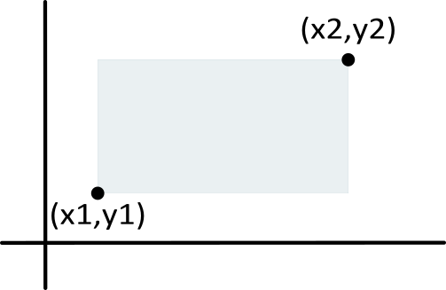
rect()function simply takes two sets of coordinatesx1,y1,x2,y2that define a rectangle. Withcolandborderyou can set the fill and border colors. For plots with many fine-scale rectangles (see later), I usually remove the border to improve details.
Next, with the `polygon()' function, we can map the alignment connections between the sequences of H. melpomene (target) and H. erato (query).
polygon(x = c(miniMap_out$targetStart[1], miniMap_out$targetEnd[1], miniMap_out$queryEnd[1], miniMap_out$queryStart[1]),
      y = c(8,8,2,2),
      col = adjustcolor('black', alpha.f = 0.1), border = FALSE)
# Assigning [1] behind the vectors extracts only the first element from it. When we plot all the matches, we will loop through these vectors using the variable [e].
The
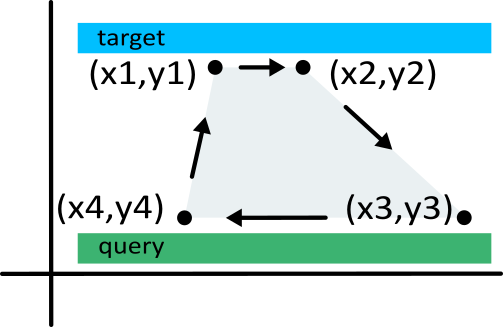
polygon()function takes sets of coordinates that define a polygon in clockwise fashion, in this casex = c(x1,x2,x3,x4)andy = c(y1,y2,y3,y4)(but you can create much more complex shapes if you'd want). See the figure below how these coordinates match the alignment coordinates in the target and query sequence. Again, withcolandborderyou can set the fill and border colors. For plots with many fine-scale polygons (see later), I usually remove the border to improve details. Note that rect() takesborder = NAwhile Polygon() takesborder = FALSE.
4.4. Plot all Minimap2 matches
We can replace the last piece of code to plot a single polygon with a loop that goes through each row in the Minimap2 alignment table and plots each match as a polygon.
for(e in 1:nrow(miniMap_out)){

  polygon(x = c(miniMap_out$targetStart[e], miniMap_out$targetEnd[e], miniMap_out$queryEnd[e], miniMap_out$queryStart[e]),
          y = c(8,8,2,2),
          col = adjustcolor('black', alpha.f = 0.1), border = FALSE)
}
The
adjustcolor()function allows to give colors somealpha.ftransparency.
4.5. Modify relative alignment
Let's make sure optix is aligned at the center of the plot between the two species. We can do this by calculating the offset of the optix positions in both fasta sequences and adjusting the coordinates in one of the two species' sequences.
# First define x-axis coordinates. This will help us later define the genomic window (xlim) we want to zoom in on.
start = 0
end = 3000000

# Calculate the offset between the positions of optix in the two fasta sequences.
# We will use this to modify all the x-axes coordinates for H. melpomene.
plotDiff = 1251211 - 706407

# Plot an empty plot (so we can fill it with rectangles (~genome) and polygons (~alignments)).
# For the y-axis (ylim) coordinates I arbitrarily use c(0,10).
plot(NULL, xlim = c(start, end), ylim = c(0,10), axes=F, ylab = '', xlab = '')

# Now we can draw two simple rectangles, one will define the genomic interval/sequence of H. melpomene (deepskyblue), the other H. erato (mediumseagreen).
rect(0+plotDiff,8,2000000+plotDiff,9, col = 'deepskyblue', border = NA)
rect(0,1,2000000,2, col = 'mediumseagreen', border = NA)

# We also know the positions of the optix gene and we can add these with the same rect() function trick.
rect(705604+plotDiff,9.2,706407+plotDiff,10, col = 'red', border = 'red') # position optix melpomene (only has one exon)

rect(1239943,0,1239972,0.8, col = 'red', border = 'red') # first exon position optix erato
rect(1250591,0,1251211,0.8, col = 'red', border = 'red') # second exon position optix erato
rect(1239943,0.4,1251211,0.4, col = 'red', border = 'red') # A little line between the two and we have a gene model!

# With the text function, we can add the gene and species names at the appropriate coordinates.
text(706407+plotDiff, 9.6, substitute(paste(italic('optix'))), pos = 4)
text(1251211, 0.4, substitute(paste(italic('optix'))), pos = 4)

text(start, 7.5, substitute(paste(italic('H. melpomene'))), pos = 4)
text(start, 2.5, substitute(paste(italic('H. erato'))), pos = 4)

# Plot the polygons representing the alignments.
for(e in 1:nrow(miniMap_out)){

  polygon(x = c(miniMap_out$targetStart[e]+plotDiff, miniMap_out$targetEnd[e]+plotDiff, miniMap_out$queryEnd[e], miniMap_out$queryStart[e]),
          y = c(8,8,2,2),
          col = adjustcolor('black', alpha.f = 0.1), border = FALSE)
}
4.6. Zoom in
As an exercise we can now try zooming in on 10,000 bp before and 200,000 bp after the start of the optix gene.
But before we do this, let's build a more complex layout of our plot first. The layout() function will help us building the panels for a complex figure layout. Here, I build one with 7 rows (nrows), each with a different height. Everytime we will call the plot() function, one panel of this layout will become filled in the order as specified in the matrix(). We will use these additional panels to add some tracks with additional genomic annotations in the next steps. More information on the layout() function can be found here.
layout(matrix(c(1,4,5,3,6,7,2), nrow=7, byrow=TRUE), height = c(0.5,1,1,2,1,1,0.5))
layout.show(n=7) # This will visualize our defined layout.

par(mar = c(0.5,5,0.5,1), xpd = FALSE) # This will set some margin settings which helps creating space for our axes labels.

# Define the interval (relative to the H. erato genome)
start = 1239943 - 10000
end = 1251211 + 200000

# Plot the title of the plot
plot(NULL, xlim=c(start,end), ylim = c(0,1), axes=FALSE, ann=FALSE)
mtext('Minimap2 aligned genome plot', side = 1, cex=1, col = 'black', line =-1)

# Plot the x-axis as a separate plot
plot(NULL, xlim=c(start,end), ylim = c(0,1), axes=FALSE, ann=FALSE)
axis(1, at = seq(0,3124353, by=10000), labels = NA, line =-3)
axis(1, at = seq(0,3124353, by=100000), labels = round(seq(0/1000000,3124353/1000000, by=0.1),1), line =-3)
mtext('Chromosome position', side = 1, cex=0.8, col = 'black', line =-1)
Now we can add the alignment polygons for a zoomed-in window to the predefined layout. We'll also add an if() statement that makes sure alignments outside of the plotting area don't get included.
# Calculate the offset between the positions of optix in the two fasta sequences.
# We will use this to modify all the x-axes coordinates for H. melpomene.
plotDiff = 1251211 - 706407

# Plot an empty plot (so we can fill it with rectangles (~genome) and polygons (~alignments)).
# For the y-axis (ylim) coordinates I arbitrarily use c(0,10).
plot(NULL, xlim = c(start, end), ylim = c(0,10), axes=F, ylab = '', xlab = '')

# Now we can draw two simple rectangles, one will define the genomic interval/sequence of H. melpomene (deepskyblue), the other H. erato (mediumseagreen).
rect(0+plotDiff,8,2000000+plotDiff,8.8, col = 'deepskyblue', border = NA)
rect(0,1.2,2000000,2, col = 'mediumseagreen', border = NA)

# We also know the positions of the optix gene and we can add these with the same rect() function trick.
rect(705604+plotDiff,9.2,706407+plotDiff,10, col = 'red', border = 'red') # position optix melpomene (only has one exon)

rect(1239943,0,1239972,0.8, col = 'red', border = 'red') # first exon position optix erato
rect(1250591,0,1251211,0.8, col = 'red', border = 'red') # second exon position optix erato
rect(1239943,0.4,1251211,0.4, col = 'red', border = 'red') # A little line between the two and we have a gene model!

# With the text function, we can add the gene and species names at the appropriate coordinates.
text(706407+plotDiff, 9.6, substitute(paste(italic('optix'))), pos = 4)
text(1251211, 0.4, substitute(paste(italic('optix'))), pos = 4)

text(start, 7.5, substitute(paste(italic('H. melpomene'))), pos = 4)
text(start, 2.5, substitute(paste(italic('H. erato'))), pos = 4)

# Plot the polygons representing the alignments.
for(e in 1:nrow(miniMap_out)){

  # I add here a filter so that alignments outside of the plotting area don't get included.
  if(miniMap_out$targetStart[e]+plotDiff > start & miniMap_out$targetEnd[e]+plotDiff < end & miniMap_out$queryStart[e] > start & miniMap_out$queryEnd[e] < end){

    polygon(x = c(miniMap_out$targetStart[e]+plotDiff, miniMap_out$targetEnd[e]+plotDiff, miniMap_out$queryEnd[e], miniMap_out$queryStart[e]),
          y = c(8,8,2,2),
          col = adjustcolor('black', alpha.f = miniMap_out$matchingBases[e]/miniMap_out$matchLength[e]), border = FALSE)

  }
}

mtext('Minimap2 alignment', side = 2, cex=0.8, padj = -1, col = 'black')
The
alpha.fvalue in theadjustcolor()function has been set here to the identity value of the alignment (i.e. (number of matching bases)/(alignment length)).With the
startandendvariable you can now zoom in on any part of the aligned.
Now that we're done with plotting the alignment, we can try adding some additional tracks with genomic information or annotations.
4.7. Add transposable element annotations
We can plot Transposable Element (TE) annotations on top of this. The TE annotations we will plot are the output of RepeatModeler. You can download the files here.
# Load the TE tables (only the columns that are relevant to us).
TE_erato <- read.table('TEs/H_erato_1801_TE.txt', header = FALSE)[,c(2,5:7)]
TE_melp <- read.table('TEs/H_melp_18003_TE.txt', header = FALSE)[,c(2,5:7)]

# Fix the column names
colnames(TE_erato) <- c('subs','scaf', 'start', 'end')
colnames(TE_melp) <- c('subs','scaf', 'start', 'end')

# (optional) remove TEs with large number of substitutions compared to database
TE_erato <- subset(TE_erato, TE_erato$subs < 15)
TE_melp  <- subset(TE_melp, TE_melp$subs < 15)

# Loop through the rows and plot each TE as a small orange rectangle.

for(e in 1:nrow(TE_melp)){
  rect(TE_melp$start[e]+plotDiff,8.8,TE_melp$end[e]+plotDiff,9, col = 'orange', border = NA)
}

for(e in 1:nrow(TE_erato)){
  rect(TE_erato$start[e],1,TE_erato$end[e],1.2, col = 'orange', border = NA)
}

# Add a little text note on the plot
mtext('TE', side = 1, cex=0.8, padj = -3, las = 1, adj=1, col = 'orange')
4.8. Add ATAC-seq data tracks
As a last step, we will add some ATAC-seq data of butterfly brain and wing tissue. You can download the files here.
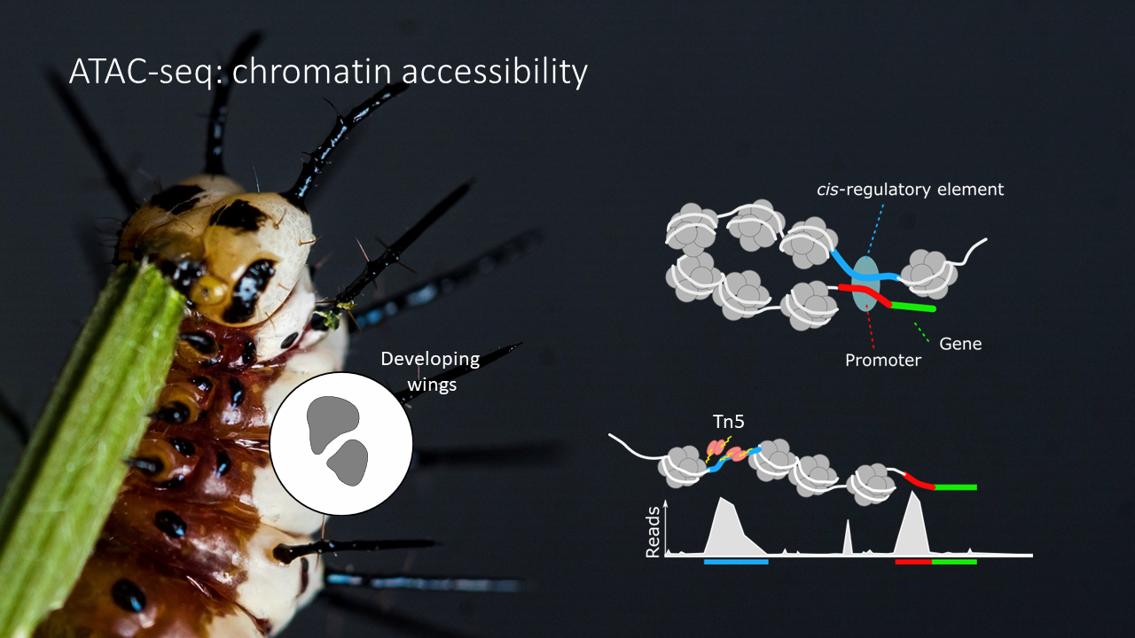
ATAC-seq (Assay for Transposase-Accessible Chromatin using sequencing) is a technique used to identify regions of chromatin that are accessible to DNA-binding proteins in a genome-wide manner. It works by using a hyperactive Tn5 transposase enzyme to insert sequencing adapters into accessible chromatin regions, which are subsequently amplified and sequenced. By comparing the resulting sequencing reads to a reference genome, we can identify regions of open chromatin and infer potential regulatory elements, such as promoters and enhancers, in a given tissue and developmental stage.
# Load the ATAC-seq data (make sure the 'rtracklayer' is loaded).

erato_5th_brain <- import.bedGraph("ATAC/brain_5th_H_erato_normalized_mean.w30s0bin.bg")
erato_5th_FW <- import.bedGraph("ATAC/FW_5th_H_erato_normalized_mean.w30s0bin.bg")

melp_5th_brain <- import.bedGraph("ATAC/brain_5th_H_melp_normalized_mean.w30s0bin.bg")
melp_5th_FW <- import.bedGraph("ATAC/FW_5th_H_melp_normalized_mean.w30s0bin.bg")
The files we are loading are called
bedgraphfiles. They simply include a summary of the amount of cut-sites resulting from the ATAC-seq protocol (summarized in intervals that have the same amount of cut sites (e.g. | scaffold | start | end | count |)). Note that for bigger datasets we would use so-calledbigwigfiles, which is a compressed alternative to the bedgraph format.
# Sample 1

# Plot an empty plot (remember, this will fill a panel defined by the layout function).
plot(NULL, xlim=c(start,end), ylim = c(0,200), axes=FALSE, ann=FALSE)
# Tell R the next plot call will be to the one that is already there and not initiate a new one.
par(new = TRUE)
# Plot the ATAC-seq track.
plot(0.5*(start(melp_5th_brain) + end(melp_5th_brain))+plotDiff, melp_5th_brain$score, type='l', xlim = c(start,end), ylim = c(0,200), ylab = "", yaxt = "n", lwd = 1, xlab = "", xaxt = "n", main = "", bty='none', col = "black")

# Add some text specifying the stage and tissue of the sample.
mtext('ATAC-seq 5th instar brain', side = 1, cex=0.8, padj = 0, las = 1, adj=1)
# Add the y-axis labels
axis(2, at = seq(0,200, by=50), line = 1)
mtext('Score', side = 2, cex=0.8, line = 3)

# Sample 2

plot(NULL, xlim=c(start,end), ylim = c(0,200), axes=FALSE, ann=FALSE)
par(new = TRUE)
plot(0.5*(start(melp_5th_FW) + end(melp_5th_FW))+plotDiff, melp_5th_FW$score, type='l', xlim = c(start,end), ylim = c(0,200), ylab = "", yaxt = "n", lwd = 1, xlab = "", xaxt = "n", main = "", bty='none', col = "black")

mtext('ATAC-seq 5th instar FW', side = 1, cex=0.8, padj = 0, las = 1, adj=1)
axis(2, at = seq(0,200, by=50), line = 1)
mtext('Score', side = 2, cex=0.8, line = 3)

# Sample 3

plot(NULL, xlim=c(start,end), ylim = c(0,200), axes=FALSE, ann=FALSE)
par(new = TRUE)
plot(0.5*(start(erato_5th_brain) + end(erato_5th_brain)), erato_5th_brain$score, type='l', xlim = c(start,end), ylim = c(0,200), ylab = "", yaxt = "n", lwd = 1, xlab = "", xaxt = "n", main = "", bty='none', col = "black")

mtext('ATAC-seq 5th instar brain', side = 1, cex=0.8, padj = 0, las = 1, adj=1)
axis(2, at = seq(0,200, by=50), line = 1)
mtext('Score', side = 2, cex=0.8, line = 3)

# Sample 4

plot(NULL, xlim=c(start,end), ylim = c(0,200), axes=FALSE, ann=FALSE)
par(new = TRUE)
plot(0.5*(start(erato_5th_FW) + end(erato_5th_FW)), erato_5th_FW$score, type='l', xlim = c(start,end), ylim = c(0,200), ylab = "", yaxt = "n", lwd = 1, xlab = "", xaxt = "n", main = "", bty='none', col = "black")

mtext('ATAC-seq 5th instar FW', side = 1, cex=0.8, padj = 0, las = 1, adj=1)
axis(2, at = seq(0,200, by=50), line = 1)
mtext('Score', side = 2, cex=0.8, line = 3)
We're done! You should now see the figure that was at the top of this tutorial.